Causal Tracing (ROME)#
Causal tracing was a methodology for locating where facts are stored in transformer LMs, introduced in the paper “Locating and Editing Factual Associations in GPT” (Meng et al., 2023). In this notebook, we will implement their method using this library and replicate the first causal tracing example in the paper (full figure 1 on page 2).
![]()
__author__ = "Aryaman Arora"
__version__ = "11/08/2023"
Set-up#
try:
    # This library is our indicator that the required installs
    # need to be done.
    import pyvene

except ModuleNotFoundError:
    !pip install git+https://github.com/stanfordnlp/pyvene.git
import torch
import pandas as pd
import numpy as np
from pyvene import embed_to_distrib, top_vals, format_token
from pyvene import (
    IntervenableModel,
    VanillaIntervention, Intervention,
    RepresentationConfig,
    IntervenableConfig,
    ConstantSourceIntervention,
    LocalistRepresentationIntervention
)
from pyvene import create_gpt2

%config InlineBackend.figure_formats = ['svg']
from plotnine import (
    ggplot,
    geom_tile,
    aes,
    facet_wrap,
    theme,
    element_text,
    geom_bar,
    geom_hline,
    scale_y_log10,
    xlab, ylab, ylim,
    scale_y_discrete, scale_y_continuous, ggsave
)
from plotnine.scales import scale_y_reverse, scale_fill_cmap
from tqdm import tqdm

titles={
    "block_output": "single restored layer in GPT2-XL",
    "mlp_activation": "center of interval of 10 patched mlp layer",
    "attention_output": "center of interval of 10 patched attn layer"
}

colors={
    "block_output": "Purples",
    "mlp_activation": "Greens",
    "attention_output": "Reds"
}
Factual recall#
Let’s set up the model (gpt2-xl) and test it on the fact we want to causal trace: “The Space Needle is in downtown Seattle”.
device = "cuda:0" if torch.cuda.is_available() else "cpu"
config, tokenizer, gpt = create_gpt2(name="gpt2-xl")
gpt.to(device)

base = "The Space Needle is in downtown"
inputs = [
    tokenizer(base, return_tensors="pt").to(device),
]
print(base)
res = gpt(**inputs[0])
distrib = embed_to_distrib(gpt, res.last_hidden_state, logits=False)
top_vals(tokenizer, distrib[0][-1], n=10)
loaded model
The Space Needle is in downtown
_Seattle             0.9763794541358948
_Bellev              0.0027682818472385406
_Portland            0.0021577849984169006
,                    0.0015149445971474051
_Vancouver           0.0014351375866681337
_San                 0.0013575783232226968
_Minneapolis         0.000938268203753978
.                    0.0007443446083925664
_Tacoma              0.0006097281584516168
_Washington          0.0005885555874556303
Corrupted run#
The first step in implementing causal tracing is to corrupt the input embeddings for the subject tokens by adding Gaussian noise to them. In Meng et al., the standard deviation of the Gaussian we sample from is computed as thrice the standard deviation of embeddings over a big dataset. We encode this as a constant, self.noise_level.
Note that the source argument is ignored unlike in causal interventions, since we are adding noise without reference to any other input.
Our intervention config intervenes on the block_input of the 0th layer, i.e. the embeddings.
class NoiseIntervention(ConstantSourceIntervention, LocalistRepresentationIntervention):
    def __init__(self, embed_dim, **kwargs):
        super().__init__()
        self.interchange_dim = embed_dim
        rs = np.random.RandomState(1)
        prng = lambda *shape: rs.randn(*shape)
        self.noise = torch.from_numpy(
            prng(1, 4, embed_dim)).to(device)
        self.noise_level = 0.13462981581687927

    def forward(self, base, source=None, subspaces=None):
        base[..., : self.interchange_dim] += self.noise * self.noise_level
        return base

    def __str__(self):
        return f"NoiseIntervention(embed_dim={self.embed_dim})"


def corrupted_config(model_type):
    config = IntervenableConfig(
        model_type=model_type,
        representations=[
            RepresentationConfig(
                0,              # layer
                "block_input",  # intervention type
            ),
        ],
        intervention_types=NoiseIntervention,
    )
    return config
Let’s check that this reduced the probability of the output “_Seattle”.
base = tokenizer("The Space Needle is in downtown", return_tensors="pt").to(device)
config = corrupted_config(type(gpt))
intervenable = IntervenableModel(config, gpt)
_, counterfactual_outputs = intervenable(
    base, unit_locations={"base": ([[[0, 1, 2, 3]]])}
)
distrib = embed_to_distrib(gpt, counterfactual_outputs.last_hidden_state, logits=False)
top_vals(tokenizer, distrib[0][-1], n=10)
_Los                 0.03294256329536438
_San                 0.03194474056363106
_Seattle             0.026176469400525093
_Toronto             0.02585919387638569
_Chicago             0.024749040603637695
_Houston             0.024224288761615753
_Atlanta             0.01866454817354679
_Austin              0.017735302448272705
_St                  0.017606761306524277
_Denver              0.01740877516567707
Restored run#
We now make a config that performs the following:
Corrupt input embeddings for some positions.
Restore the hidden state at a particular layer for some (potentially different positions).
This is how Meng et al. check where in the model the fact moves through.
def restore_corrupted_with_interval_config(
    layer, stream="mlp_activation", window=10, num_layers=48):
    start = max(0, layer - window // 2)
    end = min(num_layers, layer - (-window // 2))
    config = IntervenableConfig(
        representations=[
            RepresentationConfig(
                0,       # layer
                "block_input",  # intervention type
            ),
        ] + [
            RepresentationConfig(
                i,       # layer
                stream,  # intervention type
        ) for i in range(start, end)],
        intervention_types=\
            [NoiseIntervention]+[VanillaIntervention]*(end-start),
    )
    return config
Now let’s run this over all layers and positions! We will corrupt positions 0, 1, 2, 3 (“The Space Needle”, i.e. the subject of the fact) and restore at a single position at every layer.
# should finish within 1 min with a standard 12G GPU
token = tokenizer.encode(" Seattle")[0]
print(token)
7312
for stream in ["block_output", "mlp_activation", "attention_output"]:
    data = []
    for layer_i in tqdm(range(gpt.config.n_layer)):
        for pos_i in range(7):
            config = restore_corrupted_with_interval_config(
                layer_i, stream,
                window=1 if stream == "block_output" else 10
            )
            n_restores = len(config.representations) - 1
            intervenable = IntervenableModel(config, gpt)
            _, counterfactual_outputs = intervenable(
                base,
                [None] + [base]*n_restores,
                {
                    "sources->base": (
                        [None] + [[[pos_i]]]*n_restores,
                        [[[0, 1, 2, 3]]] + [[[pos_i]]]*n_restores,
                    )
                },
            )
            distrib = embed_to_distrib(
                gpt, counterfactual_outputs.last_hidden_state, logits=False
            )
            prob = distrib[0][-1][token].detach().cpu().item()
            data.append({"layer": layer_i, "pos": pos_i, "prob": prob})
    df = pd.DataFrame(data)
    df.to_csv(f"./tutorial_data/pyvene_rome_{stream}.csv")
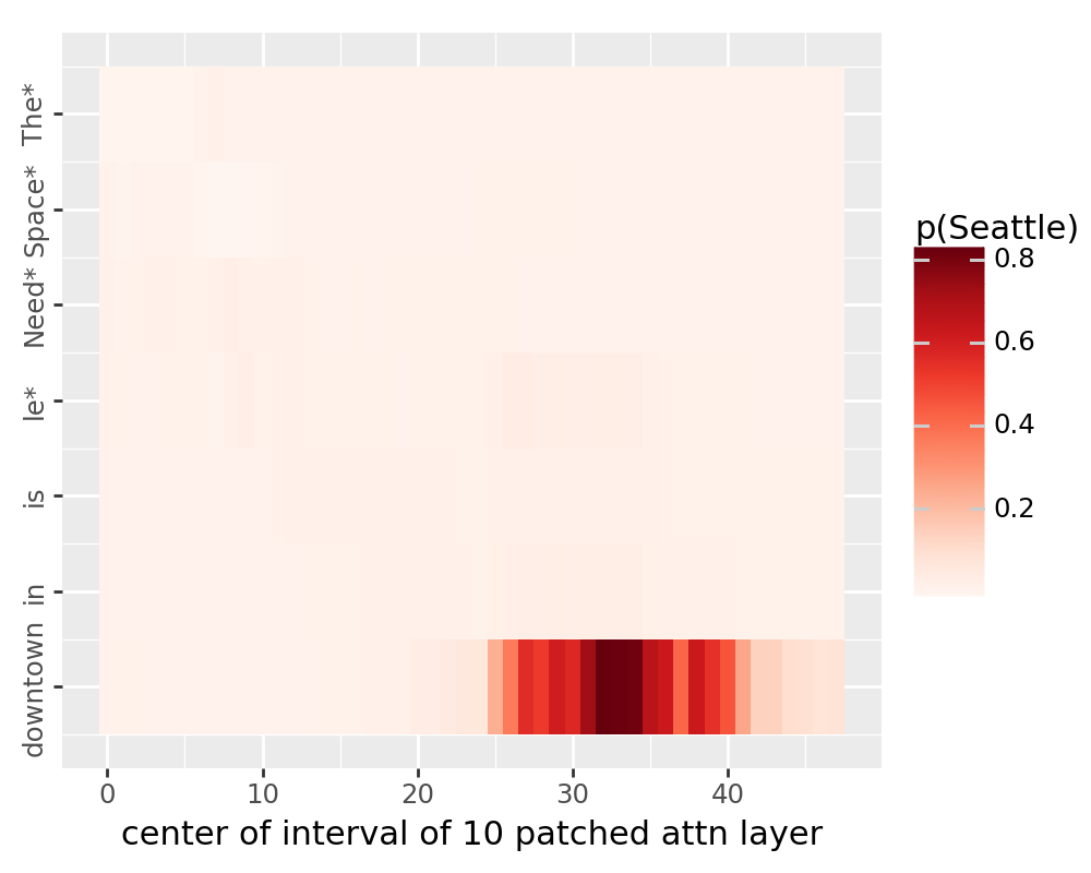
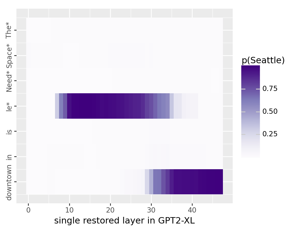
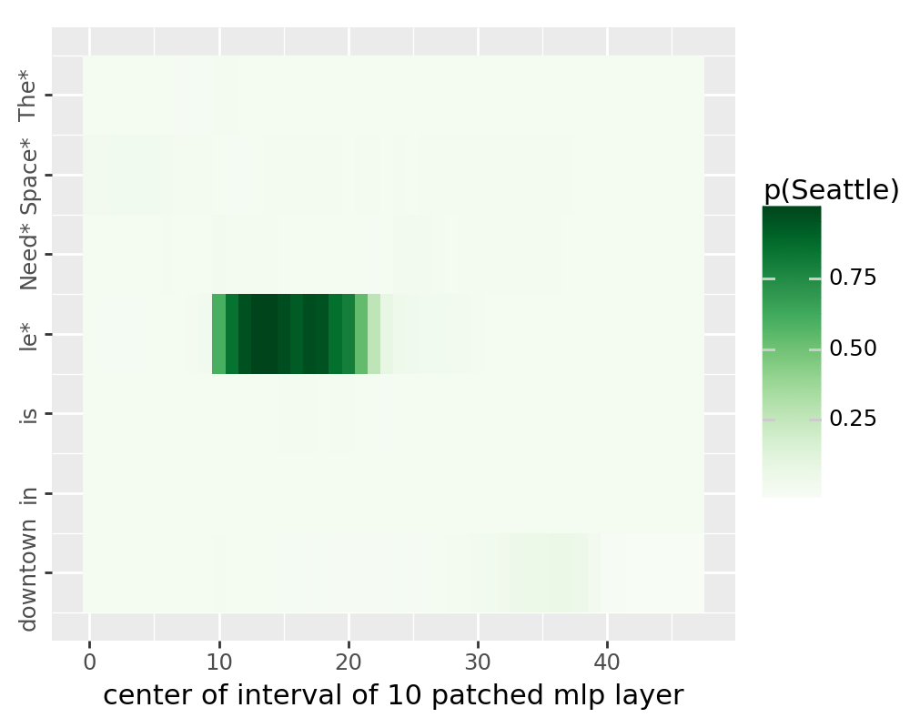
The plot below should now replicate Meng et al.
for stream in ["block_output", "mlp_activation", "attention_output"]:
    df = pd.read_csv(f"./tutorial_data/pyvene_rome_{stream}.csv")
    df["layer"] = df["layer"].astype(int)
    df["pos"] = df["pos"].astype(int)
    df["p(Seattle)"] = df["prob"].astype(float)

    custom_labels = ["The*", "Space*", "Need*", "le*", "is", "in", "downtown"]
    breaks = [0, 1, 2, 3, 4, 5, 6]

    plot = (
        ggplot(df, aes(x="layer", y="pos"))

        + geom_tile(aes(fill="p(Seattle)"))
        + scale_fill_cmap(colors[stream]) + xlab(titles[stream])
        + scale_y_reverse(
            limits = (-0.5, 6.5),
            breaks=breaks, labels=custom_labels)
        + theme(figure_size=(5, 4)) + ylab("")
        + theme(axis_text_y  = element_text(angle = 90, hjust = 1))
    )
    ggsave(
        plot, filename=f"./tutorial_data/pyvene_rome_{stream}.pdf", dpi=200
    )
    print(plot)
/u/nlp/anaconda/main/anaconda3/envs/wuzhengx-bootleg/lib/python3.8/site-packages/plotnine/ggplot.py:587: PlotnineWarning: Saving 5 x 4 in image.
/u/nlp/anaconda/main/anaconda3/envs/wuzhengx-bootleg/lib/python3.8/site-packages/plotnine/ggplot.py:588: PlotnineWarning: Filename: ./tutorial_data/pyvene_rome_block_output.pdf
/u/nlp/anaconda/main/anaconda3/envs/wuzhengx-bootleg/lib/python3.8/site-packages/plotnine/ggplot.py:587: PlotnineWarning: Saving 5 x 4 in image.
/u/nlp/anaconda/main/anaconda3/envs/wuzhengx-bootleg/lib/python3.8/site-packages/plotnine/ggplot.py:588: PlotnineWarning: Filename: ./tutorial_data/pyvene_rome_mlp_activation.pdf
/u/nlp/anaconda/main/anaconda3/envs/wuzhengx-bootleg/lib/python3.8/site-packages/plotnine/ggplot.py:587: PlotnineWarning: Saving 5 x 4 in image.
/u/nlp/anaconda/main/anaconda3/envs/wuzhengx-bootleg/lib/python3.8/site-packages/plotnine/ggplot.py:588: PlotnineWarning: Filename: ./tutorial_data/pyvene_rome_attention_output.pdf